Building an SIR Model

camdl (the Compartmental Model Description Language, pronounced “cam-dee-ell”, or rhymes with “candle”) is a domain-specific language for stochastic epidemiological compartmental models. Like SQL for databases, camdl separates the scientific declaration of a model from the code that implements it. The math is the model — what you write in a .camdl file is designed to read like the model specification and equations you’d put on a whiteboard. Other modeling frameworks often force you to write code that blends the declaration of the scientific model with implementation code; camdl intentionally keeps them apart. Moreover, camdl has a compiler that actually checks the semantics and validity of your scientific model before simulating from it, which eliminates whole classes of bugs that come from writing code that blends the scientific model with the computational implementation.

To see what this means in practice, we start with the “Hello, World!” of epidemiology: the SIR model, nearly 100 years old, first described by Kermack and McKendrick (1927).

The SIR model divides a population into three compartments: Susceptible individuals who can catch the disease, Infected individuals who can transmit it, and Removed individuals who have recovered (or died) and play no further role. Susceptibles become infected at a propensity proportional to the contact rate \(\beta\) between \(S\) and \(I\); infected individuals recover at a constant per-capita rate \(\gamma\). Thus, two parameters govern the dynamics: the transmission rate \(\beta\) and the recovery rate \(\gamma\). We write out both the model dynamic equations and camdl code below (don’t fret if you don’t follow the math notation):

The math

Compartments: \(S\), \(I\), \(R\)

Parameters: \(\beta\) (transmission rate), \(\gamma\) (recovery rate), \(N_0\) (population size), \(I_0\) (initial infections)

Dynamics: \[ \begin{aligned} \frac{dS}{dt} &= -\beta \frac{SI}{N} \\[4pt] \frac{dI}{dt} &= \beta \frac{SI}{N} - \gamma I \\[4pt] \frac{dR}{dt} &= \gamma I \end{aligned} \]

Initial conditions: \(S(0) = N_0 - I_0, \quad I(0) = I_0\)

The code

compartments { S, I, R }

parameters {
  beta  : rate
  gamma : rate
  N0    : count
  I0    : count
}

let N = S + I + R

transitions {
  infection : S --> I  @ beta * S * I / N
  recovery  : I --> R  @ gamma * I
}

init {
  S = N0 - I0
  I = I0
}

That’s the complete camdl code for an SIR model! Let’s run it, then walk through what each piece does.

TipThis is deliberately simple

The SIR model here treats everyone as identical — one population, no age groups, no spatial structure. Real models need more: age-stratified contact matrices, spatial patches loaded from census data, partial stratification for vaccination status. camdl supports all of this through its dimension and table system, with compiler-checked type safety on every index. Start here to learn the syntax; the complexity scales when you need it.

Run it, see it

The full model and parameter files for this chapter are in guide/getting-started/. Clone the book repo and cd into that directory to follow along.

Running camdl simulate without arguments shows the help — a quick reference for what’s available:

$ camdl simulate
error: the following required arguments were not provided:
  <MODEL>

Usage: camdl simulate <MODEL>

For more information, try '--help'.

Don’t worry about the advanced flags yet — we’ll use most of them through this guide. For now, the basic invocation:

camdl simulate sir.camdl \
  --param beta=0.4 --param gamma=0.15 \
  --param N0=10000 --param I0=10 \
  --seed 42

t	S	I	R	flow_infection	flow_recovery
0	9990	10	0	0	0
1	9986	9	5	4	5
2	9982	10	8	4	3
3	9977	13	10	5	2
4	9968	20	12	9	2
5	9963	21	16	5	4
6	9954	27	19	9	3
7	9945	32	23	9	4
8	9934	38	28	11	5
9	9922	45	33	12	5

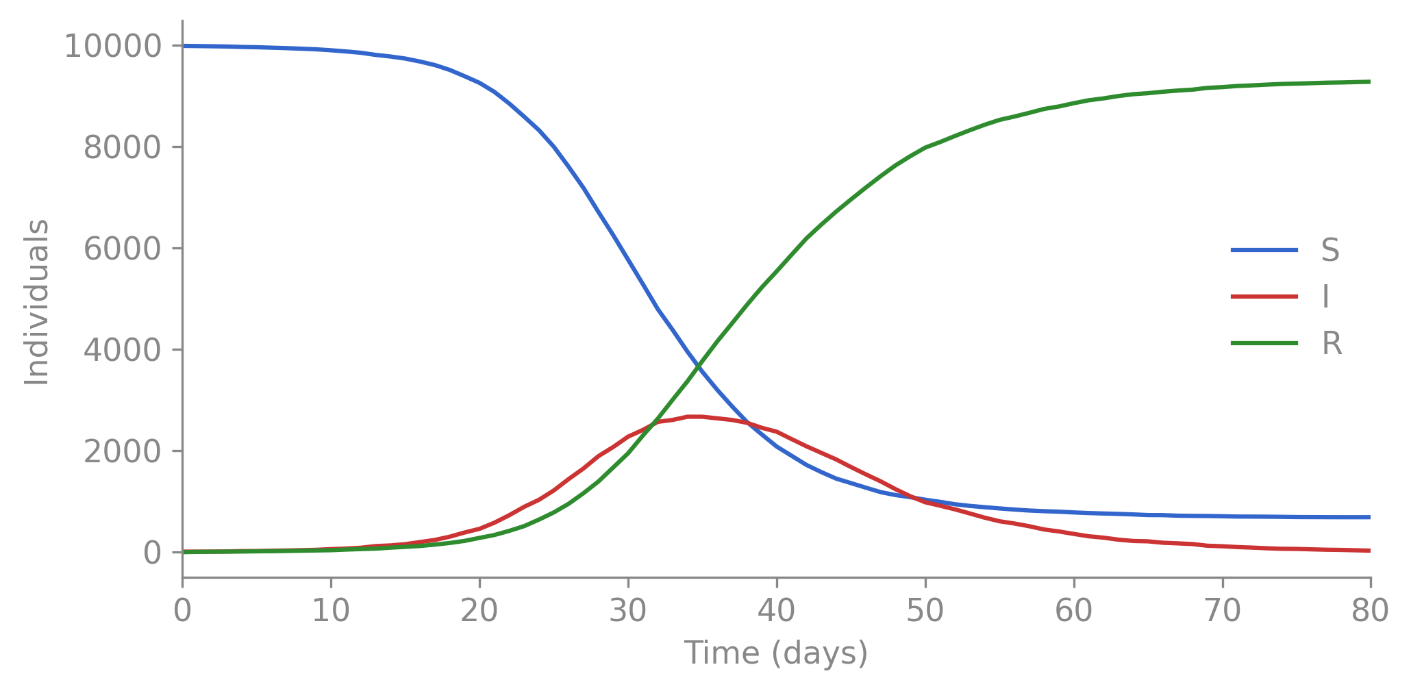
import polars as pl
import matplotlib.pyplot as plt

# df = pl.read_csv("output.tsv", separator="\t")  # from: camdl simulate sir.camdl ...
fig, ax = plt.subplots(figsize=(7, 3.5))
for col, color in [("S", "#3366cc"), ("I", "#cc3333"), ("R", "#2e8b2e")]:
    ax.plot(df["t"], df[col], color=color, label=col, linewidth=1.5)
ax.set_xlabel("Time (days)")
ax.set_ylabel("Individuals")
ax.legend(frameon=False)
ax.set_xlim(0, df["t"].max())
ax.spines[["top", "right"]].set_visible(False)
plt.tight_layout()
plt.show()

Figure 2.1: A single stochastic SIR trajectory. S declines as infection spreads, I rises and falls, R accumulates.

In 16 lines of camdl, we defined a stochastic SIR epidemic. The rest of this chapter explains what those 16 lines mean, why camdl’s syntax is designed this way, and additional model language features that lead to better readability, correctness, and easier downstream inference when we don’t know the parameters and want to fit the model to data.

Compartments — defining what exists

A key unifying feature of many epidemological models is to take the immense complexity of human immunity and disease progression and reduce it to a few discrete states that capture the key epidemiological dynamics. The compartments block defines these states. In SIR, there are three compartments,

compartments { S, I, R }

These three compartments are integer counts that partition the population’s immunological states at any given time. The camdl simulation runtime advances the epidemic by moving individuals between these compartments according to the transitions we’ll define shortly — but first, we need to declare the model’s parameters.

Parameters

A camdl model separates the model structure (compartments, transitions, observation process) from the model parameterization (the specific numeric values that govern its behavior). The parameters block declares what the model’s degrees of freedom are — the knobs you turn. By design, camdl does not support default values in the parameters block. You always supply parameter values externally, either through a TOML file or at the command line. This keeps the model definition clean: the .camdl file says what the model is, not what any particular run of it looks like.

NoteWhy no default parameter values?

This is an intentional design choice inspired by the Stan ecosystem’s philosophy. As Betancourt (2018) puts it:

[Principled modeling choices are] informed by sincere and careful deliberation, in contrast to choices informed by unquestioned defaults that have ossified into convention.

Default parameters in scientific software create implicit assumptions that silently propagate when models are shared, adapted, or applied to new pathogens. Stan’s developers learned this the hard way from BUGS and JAGS, where example models used vague priors like dnorm(0, 0.001) that users cargo-culted without understanding their implications (Gelman, 2006; Carpenter et al., 2017). When camdl refuses to simulate without a value for \(\gamma\), it’s forcing a choice you’d have to make anyway — and making that choice visible to anyone who reads the model.

Every parameter in camdl has a type that says what kind of quantity it is. These parameter types serve two purposes: they document the mathematical and scientific meaning of the parameter (e.g., it helps readers understand and better intuit a model if they can see that beta is a rate and rho is a probability), and the type tells the compiler what values are correct versus incorrect. For example, a rate can’t be negative, a probability can’t be 1.5, and a count can’t be 3.7.

The compiler enforces these constraints, and during inference, camdl uses these parameter types to choose the right parameter transform (log for rates, logit for probabilities) so the sampler explores an unconstrained space while the model always sees valid values.

Here is a parameter block with types:

parameters {
  beta  : rate                        # ≥ 0, units of 1/time
  gamma : rate                        # ≥ 0, units of 1/time
  N0    : count                       # non-negative integer
  I0    : count                       # non-negative integer
}

There are four built-in parameter types in camdl:

Table 2.1: Parameter types and their domains.

Type	Domain	Example use
rate	\([0, \infty)\)	transmission, recovery
probability	\([0, 1]\)	reporting fraction
positive	\((0, \infty)\)	\(R_0\), dispersion
count	\(\{0, 1, 2, \ldots\}\)	population, initial seed

You’ll see more on why this matters in Fitting to Data; getting the types right means camdl can fit your model without you having to think about parameter transforms — the compiler naturally knows what is best to use as a result of the parameter you declare.

Bounds

Types constrain the domain; bounds narrow it further for a specific model. beta : rate means “non-negative.” Adding in [0.01, 2.0] means “non-negative, and for this model we only consider values between 0.01 and 2.0.” Often you have scientific knowledge that rules out certain parameter values (e.g. the common cold does not have an \(R_0 = 100\)), and adding bounds helps the compiler and inference algorithms focus on the relevant region of parameter space (which can greatly improve model fitting performance). Bounds also serve as documentation for readers, showing the range of plausible values, in much the same way that parameter types do.

Here is an example of parameters with bounds:

parameters {
  beta  : rate  in [0.01, 2.0]
  gamma : rate  in [0.01, 1.0]
}

Bounds are optional for simulation-only models, but required for inference — they define the feasible region the fitting algorithms search over.

Unit literals

A pervasive source of bugs in epidemic modeling (and scientific software more generally) is unit mismatch. By design, camdl supports unit annotations on numeric literals, and the compiler automatically converts between units to match the model’s time_unit (which is by default the 'day but can be configured in the .camdl file).

For example, suppose a paper reports a mortality rate of 20 per 100,000 per year. You type 0.0002 thinking “per day,” but you forgot to divide by 365… or are there 365.25 days in a year to handle leap years? Or is it 365.2425? These are the type of subtle, difficult-to-spot bugs that come from manual unit conversion and cause serious problems.

To prevent these issues, camdl supports unit literals — tick-prefixed annotations like 'days, 'weeks, 'per_day, 'per_year — that tell the compiler what units a number is in. The compiler converts everything to the model’s time_unit automatically. Our initial SIR model omitted the time_unit declaration (it defaults to 'days), but here’s how unit literals work in practice:

time_unit = 'days

# A paper reports mortality as 20 per 100,000 per year.
# Parentheses apply the unit to the whole expression.
let mu : rate = (20 / 100_000) 'per_year

simulate {
  from = 0 'days
  to   = 12 'weeks                    # compiler converts: 84 days
}

observations {
  cases : {
    projected = incidence(infection)
    every = 1 'weeks                  # weekly reporting
    ...
  }
}

(20 / 100_000) 'per_year and 0.000000548 'per_day are the same rate — the compiler handles the conversion, and the unit annotation documents where the number came from. The parentheses matter: a unit literal binds to the number immediately before it, so 20 / 100_000 'per_year would apply 'per_year only to 100_000, not to the whole expression. Rather than silently picking the wrong interpretation, the compiler refuses with a hard error that points at the exact span and tells you the fix:

$ camdl check bad.camdl   # 20 / 100_000 'per_year (no parens)
error[E107]: ambiguous unit literal after '/': the unit suffix binds to the adjacent number, not the whole expression. Use parentheses: (20 / 100_000) 'per_year, or pre-compute: 0.0002 'per_year

  ┌─ /var/folders/mp/j_ybkq8j72ndvhfm_1msdj1c0000gn/T/camdl_paren_rtl5vosp/bad.camdl:8:17
  │
  8│  let mu : rate = 20 / 100_000 'per_year
  │                  ~~~~~~~~~~~~~~~~~~~~~^
  │

Numeric literals also support underscore separators for readability — write 100_000 instead of 100000. The compiler even warns you if your grouping looks like a typo:

 warning[W100]: suspicious digit grouping in '10_00' (group widths: 2, 2) — did you mean 1000? Use 3-digit groups: 1_000, 10_000, 1_000_000
 
   ┌─ sir.camdl:10:12
   │
 10│  init { S = 10_00 }
   │             ~~~~^
   │
 

Transitions — what happens

Transitions are events that move individuals between compartments. Each transition event has three parts: a label (infection), an arrow (S --> I) naming the source and destination compartments, and a propensity (@ beta * S * I / N) that defines the expected number of events per unit time across the entire population.

transitions {
  infection : S --> I  @ beta * S * I / N
  recovery  : I --> R  @ gamma * I
}

The syntax of camdl is designed to make these expressions easy to read and understand — especially useful as models get longer and more complex. We can read each line as a sentence: “an infection event moves individuals from S to I at propensity \(\beta S I / N\)”; “a recovery event moves individuals from I to R at propensity \(\gamma I\).”

ImportantPropensity, not rate

The expression after @ is the propensity — the total expected number of events per unit time across the entire population. It is not the per-capita rate.

Table 2.2: Decomposing propensities into per-capita rates and populations at risk.

Transition	Per-capita rate	× Population at risk	= Propensity
infection	\(\beta I/N\)	\(S\)	\(\beta S I / N\)
recovery	\(\gamma\)	\(I\)	\(\gamma I\)

camdl never silently multiplies by a population count — explicit is safer than implicit. You write the multiplication yourself. This eliminates a common source of modeling bugs: ambiguity about whether a “rate” is per-capita or total. Some frameworks have you specify per-capita rates and the engine multiplies by the source population internally. In camdl, what you write is what you get. The @ expression is the propensity.

Let bindings — names for expressions

let N = S + I + R

This looks like a variable assignment but it isn’t. let creates a named expression — the compiler substitutes S + I + R everywhere N appears, so it’s re-evaluated with the current compartment values at every simulation step.

N always reflects the current population because the substituted expression is re-evaluated at every simulation step. If an individual moves from S to I, N stays the same (closed population) but I/N changes. Remember: let bindings are live expressions, not cached values.

A second example for readability:

let foi = beta * I / N    # force of infection

transitions {
  infection : S --> I  @ foi * S
}

foi isn’t computed once — it’s a name for the expression beta * I / N, evaluated fresh every time it appears.

Initial conditions

Every compartment starts with individuals assigned to various states at time zero. The init block defines these initial conditions. You can specify an initial values through integers,

init {
  S = N0 - I0
  I = I0
}

or you can use fractional parameters when absolute counts aren’t known. This is common in practice — a paper might report that 3% of the population was susceptible at the start of an outbreak, not that exactly 297 individuals were. In camdl, you’d write:

parameters {
  s0 : probability    # initial susceptible fraction
  i0 : probability    # initial infected fraction
  N0 : count
}

init {
  S = s0 * N0
  I = i0 * N0
  R = N0 - s0 * N0 - i0 * N0
}

Compartments not mentioned in init start at zero. R isn’t listed in our SIR example above, so \(R(0) = 0\).

Init expressions can reference parameters and do arithmetic. They’re evaluated once at \(t = 0\).

Running the model

To simulate, you need to supply every parameter declared in the model. camdl will not guess — omit one and you get a clear error listing what’s missing. The simplest approach is a TOML file:

# params.toml
beta  = 0.4
gamma = 0.15
N0    = 10000
I0    = 10

camdl simulate sir.camdl --params params.toml --seed 42

You can override individual values at the command line with --param:

camdl simulate sir.camdl --params params.toml --param beta=0.6 --seed 42

--param takes precedence over the file. Typos are caught immediately — --param bta=0.6 produces an error listing the available parameter names.

For complex workflows you can stack multiple --params files (later files override earlier ones), and --param overrides everything. This layering is useful when you have a base parameter set and want to swap in regional or pathogen-specific values without editing the original file.

To see exactly what values will be used without running a simulation, use --dry-run:

$ camdl simulate sir.camdl --params params.toml --param beta=0.6 --seed 42 --dry-run
camdl simulate (dry run)

  model: sir.camdl
  backend: chain_binomial
  dt: 1
  seed: 42
  scenario: (baseline)

Parameters (6):
  I0    =     10  params.toml
  N0    =  10000  params.toml
  beta  = 0.600000  --param (was 0.400000 in params.toml)
  gamma = 0.150000  params.toml
  k     =     10  params.toml
  rho   = 0.600000  params.toml

Every parameter shows its final value and where it came from. When a value was overridden, you can see both the new value and what it replaced — here, beta was 0.4 in params.toml but overridden to 0.6 by --param.

TipParameter precedence and error handling

camdl’s parameter resolution is designed to prevent silent mistakes:

• Missing parameters are a hard error. The error message lists exactly which parameters are missing.
• Unknown parameters (typos like bta instead of beta) are a hard error in both --param and --params files, with a list of valid names.
• Precedence follows a simple rule: later sources override earlier ones. --params files are applied left-to-right, and --param flags override everything.
• --dry-run resolves the full parameter vector and shows provenance without running any simulation — useful for verifying complex setups before committing to a long batch run.

Output is TSV on stdout — time, compartment populations, and flow accumulators. Pipe it wherever you want:

camdl simulate sir.camdl --params params.toml --seed 42 > output.tsv

Every run is stochastic — different seeds give different trajectories. Run 5 replicates and overlay the curves:

camdl simulate sir.camdl --params params.toml --seed 42 --replicates 5

With --replicates, camdl derives independent seeds from the base seed, runs multiple simulations, and stacks the results on top of each other in the output TSV, with an additional replicate column to distinguish them. The resulting file looks like:

replicate	t	S	I	R	flow_infection	flow_recovery
1	0	9990	10	0	0	0
1	1	9986	9	5	4	5
1	2	9982	10	8	4	3
1	3	9977	13	10	5	2
1	4	9968	20	12	9	2
1	5	9963	21	16	5	4
1	6	9954	27	19	9	3
1	7	9945	32	23	9	4
…

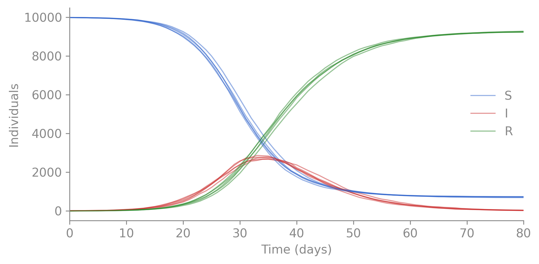
Each replicate is a full independent trajectory. Overlaying them shows the range of stochastic outcomes under the same parameters:

import polars as pl
import matplotlib.pyplot as plt

fig, ax = plt.subplots(figsize=(7, 3.5))
colors = {"S": "#3366cc", "I": "#cc3333", "R": "#2e8b2e"}
for i, d in enumerate(multi.partition_by("replicate")):
    for col, color in colors.items():
        ax.plot(d["t"], d[col], color=color, alpha=0.5, linewidth=1,
                label=col if i == 0 else None)
ax.set_xlabel("Time (days)")
ax.set_ylabel("Individuals")
ax.legend(frameon=False)
ax.set_xlim(0, d["t"].max())
ax.spines[["top", "right"]].set_visible(False)
plt.tight_layout()
plt.show()

Figure 2.2: Five stochastic SIR trajectories from different seeds. Same parameters, different realizations of the stochastic process.

This is the stochastic process from §1 of the inference guide. The latent state you never observe directly.

Observations — connecting your model to data

So far, the model describes how an epidemic unfolds. But we don’t observe the S, I, and R trajectories directly. What we actually get from a surveillance system is noisy, delayed, and incomplete: weekly case reports where only a fraction of infections are caught, and the counts bounce around from week to week even when the underlying epidemic is smooth. The observations block describes this measurement process — the pipeline that stands between the true epidemic and your data.

In our SIR model, the true number of infections each week is tracked by incidence(infection) — the flow accumulator counting S → I events since the last observation time. But surveillance systems don’t report every infection. A fraction \(\rho\) of cases are reported, and the counts are overdispersed — some weeks more cases are caught than expected, some weeks fewer. The neg_binomial likelihood captures both effects: the mean is \(\rho\) times the true incidence, and the dispersion parameter \(k\) controls how noisy the observations are around that mean.

parameters {
  rho : probability  in [0.1, 0.9]    # reporting fraction
  k   : positive     in [1.0, 100.0]  # NegBin dispersion
}

observations {
  weekly_cases : {
    projected  = incidence(infection)
    every      = 7 'days
    likelihood = neg_binomial(mean = rho * projected, r = k)
  }
}

TipIncidence vs. prevalence — events vs. states

incidence(...) and prevalence(...) are projection functions: they take a model object and produce a scalar that the likelihood can consume. They look like ordinary function calls because they are. Which one applies depends on what the data actually measures:

• incidence(transition) — a flow accumulator. It counts how many times the named transition fired between the previous observation time and this one, then resets. Use this when your data records events happening over a window — weekly case reports, monthly hospitalizations, daily deaths. Argument is a transition label (e.g. infection, recovery).

• prevalence(compartment) — an instantaneous snapshot. It returns the count of individuals in the named compartment at the observation time, no accumulation. Use this when your data records who is in what state right now — seroprevalence surveys, point-in-time hospital censuses, current-infection counts from a cross-sectional study. Argument is a compartment name (e.g. I, R).

The argument type tells you which is sensible: transitions are events and have rates; compartments are states and have populations. You wouldn’t ask “how much S happened this week?” and you wouldn’t ask “how many people are currently in the infection event?” — the two functions exist precisely so the model can speak about both.

camdl also supports arithmetic projections — any expression over compartments, parameters, and time. projected = (I + R) / N is the ever-infected fraction; projected = prevalence(I) / N0 is point prevalence as a proportion. Arithmetic projections compile to the same machinery as prevalence(...); the named form is just sugar for the single-compartment case.

A prevalence-style observation block, for the case where what you measure is “fraction of the population currently infected” (e.g. a periodic serosurvey of active infection):

observations {
  point_prevalence : {
    projected  = I / N0                     # fraction currently infected
    every      = 14 'days                   # biweekly survey
    likelihood = binomial(n = n_sampled, p = projected)
  }
}

The same model can host both blocks at once — a weekly case-report stream and a biweekly prevalence survey, each with its own likelihood. The inference engine combines the log-likelihoods automatically.

To see this pipeline in action, generate synthetic observations alongside the trajectory with the --obs flag:

camdl simulate sir.camdl --params params.toml --seed 42 --obs cases.tsv

This runs the same stochastic simulation and then draws from the neg_binomial likelihood at each observation time, writing the synthetic data to cases.tsv. The trajectory output is unchanged — the observation RNG is seeded independently, so adding --obs produces byte-identical trajectories.

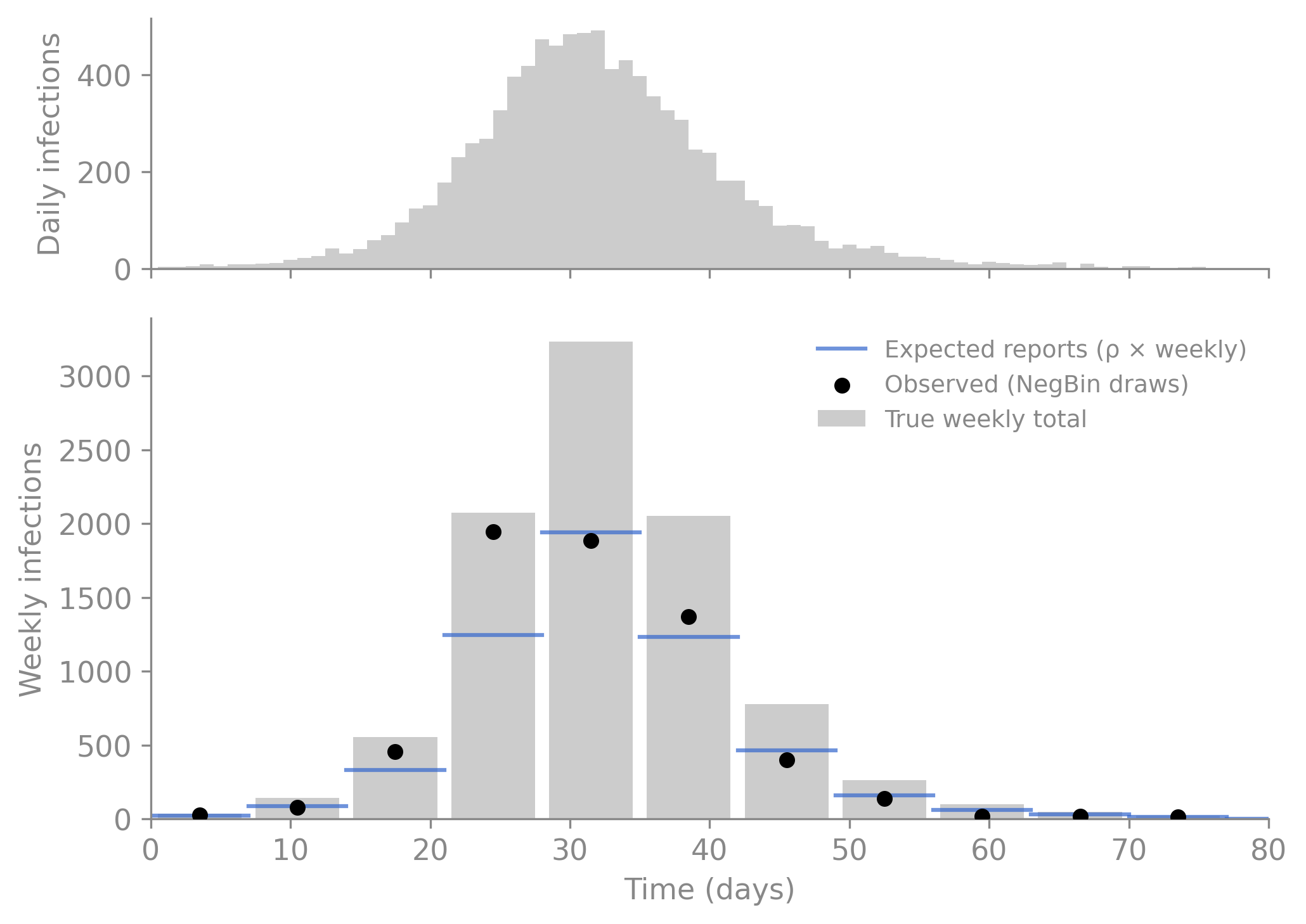
The three-layer plot below shows exactly what this pipeline does to the signal. The light grey bars are the true daily infections — what actually happened in the simulation. The stepped blue line is the expected weekly report after applying the reporting fraction \(\rho\) (here 0.6, so 60% of cases are reported). The black dots are the synthetic observations generated by --obs — negative binomial draws around that expected value, with dispersion \(k = 10\). This is the information loss that inference must invert.

import polars as pl
import matplotlib.pyplot as plt
import numpy as np

# Generate synthetic observations from the observation model
_, obs_df = run_simulate(MODEL, PARAMS, seed=42, obs=True)

# Daily new infections (flow_infection is already per-step)
daily_infections = df["flow_infection"]

# Aggregate to weekly
weeks = (df["t"] // 7).cast(pl.Int64)
weekly = (
    df.with_columns(daily_infections.alias("new_infections"), weeks.alias("week"))
    .group_by("week")
    .agg(pl.col("new_infections").sum())
    .sort("week")
)
week_starts = weekly["week"].to_numpy() * 7

# Expected reports (rho from params.toml)
rho = 0.6
true_weekly = weekly["new_infections"].to_numpy().astype(float)
expected = rho * true_weekly

# Observed counts from camdl --obs (NegBin draws from the observation model)
# Drop the t=0 row (before the first observation window completes)
obs_df = obs_df.filter(pl.col("time") > 0)
observed = obs_df["weekly_cases"].to_numpy()
obs_times = obs_df["time"].to_numpy()

fig, (ax_daily, ax_weekly) = plt.subplots(2, 1, figsize=(7, 5),
    height_ratios=[1, 2], sharex=True)

# ── Top panel: true daily incidence ──
ax_daily.bar(df["t"], daily_infections, width=1, color="#cccccc",
             edgecolor="none")
ax_daily.set_ylabel("Daily infections")
ax_daily.spines[["top", "right"]].set_visible(False)

# ── Bottom panel: weekly pipeline ──
# Layer 1: true weekly totals
ax_weekly.bar(week_starts + 3.5, true_weekly, width=6, color="#cccccc",
              edgecolor="none", label="True weekly total", zorder=1)

# Layer 2: expected weekly reports (stepped)
for i in range(len(weekly)):
    x0 = week_starts[i]
    x1 = x0 + 7
    ax_weekly.plot([x0, x1], [expected[i], expected[i]], color="#3366cc",
                   linewidth=1.5, alpha=0.7,
                   label="Expected reports (ρ × weekly)" if i == 0 else None,
                   zorder=2)

# Layer 3: observed draws from camdl --obs
ax_weekly.scatter(obs_times - 3.5, observed, color="black", s=25, zorder=3,
                  label="Observed (NegBin draws)")

ax_weekly.set_xlabel("Time (days)")
ax_weekly.set_ylabel("Weekly infections")
ax_weekly.legend(frameon=False, fontsize=9)
ax_weekly.set_xlim(0, df["t"].max())
ax_weekly.spines[["top", "right"]].set_visible(False)
plt.tight_layout()
plt.show()

Figure 2.3: The observation pipeline. Top: true daily infections from the simulation. Bottom: the same signal aggregated to weekly totals (grey bars), scaled by the reporting fraction ρ = 0.6 (blue step), and scattered by negative binomial noise (black dots). Each layer loses information; inference must recover the epidemic from only the black dots.

camdl supports multiple observation streams in a single model — for example, weekly case counts from one surveillance system and wastewater viral load from another. Each stream gets its own name, accumulator, and likelihood. We’ll see examples of this in later chapters.

This is the observation pipeline that inference must invert. Given only the black dots, the fitting algorithms in Fitting to Data will try to recover \(\beta\), \(\gamma\), and \(\rho\).

The complete first model

time_unit = 'days

compartments { S, I, R }

parameters {
  beta  : rate         in [0.05, 1.0]
  gamma : rate         in [0.01, 0.5]
  N0    : count
  I0    : count
  rho   : probability  in [0.1, 0.9]
  k     : positive     in [1.0, 100.0]
}

let N = S + I + R

transitions {
  infection : S --> I  @ beta * S * I / N
  recovery  : I --> R  @ gamma * I
}

init {
  S = N0 - I0
  I = I0
}

observations {
  weekly_cases : {
    projected  = incidence(infection)
    every      = 7 'days
    likelihood = neg_binomial(mean = rho * projected, r = k)
  }
}

simulate {
  from = 0 'days
  to   = 80 'days
}

30 lines. A stochastic SIR with typed parameters and a statistical observation model. This is the sir.camdl in guide/getting-started/, along with params.toml.

A glimpse of what’s ahead

The SIR is the simplest possible compartmental model — one pathogen, one population, no age structure. Real models need to stratify by age, spatial patch, risk group, or all three. In camdl, this is a few extra lines:

dimensions {
  age = [child, adult, elderly]
}

stratify(by = age)

tables {
  C : age × age = external("contact_matrix.csv")
}

transitions {
  infection[a in age] : S[a] --> I[a]
    @ beta * S[a] * sum(b in age, C[a, b] * I[b] / N[b])
  recovery[a in age]  : I[a] --> R[a]  @ gamma * I[a]
}

stratify(by = age) expands every compartment — S becomes S[child], S[adult], S[elderly]. Transitions are indexed over the dimension. The contact matrix C governs who infects whom. The compiler checks that all dimensions align, that the contact matrix is the right shape, and that no index is misspelled. This is the same SIR — just with age groups — and the compiler does all the bookkeeping.

We’ll cover dimensions, spatial patches, and contact matrices in a later chapter. For now, the next step is learning to ask “what if?” — comparing scenarios, running experiments, and checking whether your model’s assumptions produce plausible epidemics.

What’s next

• Uncertainty, Priors, Simulation, and Experiments — prior predictive checks, process uncertainty, and the observation model.
• Scenarios, Interventions, and Sweeps — counterfactual comparisons, parameter sweeps, and the batch system.
• Fitting to Data — recover parameters with IF2 and PGAS+NUTS.